Fred Yang, Deputy Technical Manager Product Division of CoreTech System (Moldex3D)

For the curved surfaces commonly found on polymer reinforced composite products, complex ply designs are required. Therefore, before the modeling of the resin transfer molding (RTM) process, the corresponding solid mesh must be established according to the ply setting of the product design. The mesh establishment for a complex layered surface is exceedingly difficult, so users must spend a lot of time on mesh pre-processing. Otherwise, the accuracy can be affected in the simulation results and thus the following result interpretations.

Previously, users have had to spend more time on Moldex3D mesh pre-processing for RTM. Also, the solid mesh needed to be rebuilt from very beginning for even minor changes in the runner design. Moreover, in some simulation cases, there are issues resulting in broken melt front and the abnormal internal pressure exceeding the inlet pressure. To overcome these challenges, Moldex3D 2021 Solver supports analysis with non-matching mesh. Meanwhile, the Solver’s calculation capabilities have been enhanced to eliminate the melt front and pressure issues and obtain better analysis results.

When the solver does not support non-matching meshes, as shown in Fig. 1 (a), the fully matched solid mesh has to be generated first during the pre-processing of the RTM project, t, as shown in Fig. 1 (b). Therefore, the user must check whether the meshes are completely matched and fix the corresponding mesh issues before running the analysis. Modex3D 2021 RTM solver now supports the non-matching mesh analysis, so the nodes on the interface of the solid mesh do not need to be completely matched to each other for analysis, reducing a lot of time and effort spent fixing the solid mesh.

The workflow of establishing non-matching mesh is the same as that for matching mesh. If the users want to evaluate the design changes of ply and runner, they only need to adjust the mesh partially instead of deleting and rebuilding all the mesh.

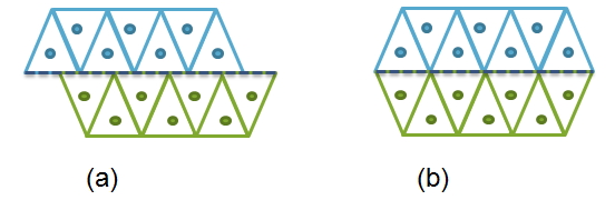
Fig. 1 (a) Non-matching mesh; (b) Matching mesh

In the following validation case, the simulation results of non-matching and matching mesh are compared. The model in this case is built through a permeability measurement instrument, Easyperm. The instrument is shown from both outside and inside in Fig. 2 (a)(b). The geometry model established based on the cavity is shown in Fig. 2(c), and SNX1, SNX2, SNY1, and SNY2are the positions of the pressure sensors inside the mold. The non-matching mesh and the simulation results are shown in Fig. 3 and Fig. 4. In the results summary of Fig. 4, NM simu and M simu are referred to in the simulation results of the non-matching and the matching mesh, respectively. According to the result comparison of the pressure change of the sensor points over time, the non-matching mesh and the matching mesh have simulation results in good agreement to each other. as can be seen in Fig. 3 (c) (d), the maximum error of the melt front time results is about 4%, and the velocity vector and the pressure field distribution are continuous at the interface inside the non-matching meshes. Through this case validation, one can see the mesh model no longer needs to be completely matched, and the simulation results can still be consistent with that obtained with fully matching mesh.

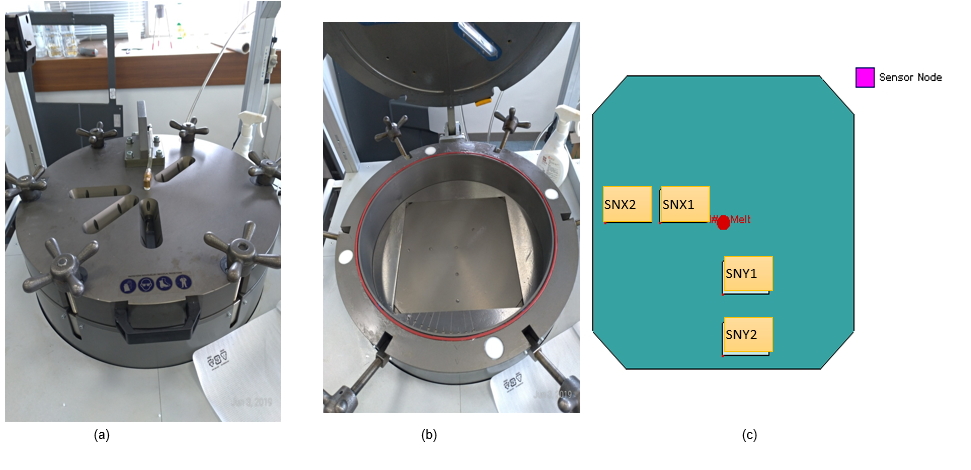
Fig. 2 (a) The Easyperm; (b) Use the Easyperm to measure the inside of the mold; (c) The geometry of the model and the position of the pressure sensor points inside the mold

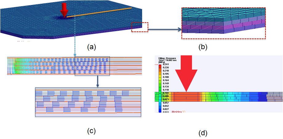
Fig. 3 (a) The mesh model in the validation case, (b) Non-matching mesh, (c) Velocity vector, (d) Pressure distribution

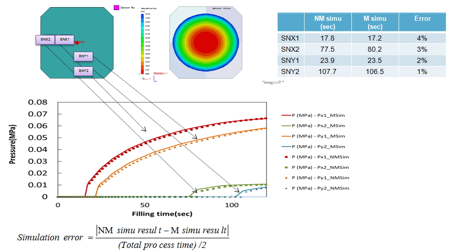
Fig. 4 The pressure variation at the sensor points and melt front time difference

In the second validation case, non-matching mesh is used to exam the result differences due to the changes of the runner position and amount. Fig. 5 shows the model arranged with one runner (a) and two runners (b), and one can see result differences in flow time (c) and melt front time (d).

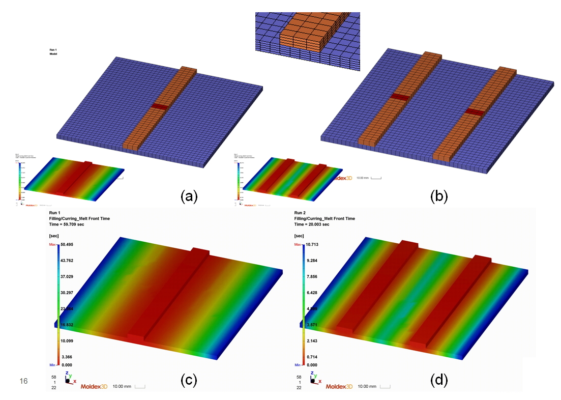
Fig. 5 (a) The mesh of one runner arrangement, (b) The mesh of two runner arrangement; (c) Melt front time results for the case of arranging one runner, (d) Melt front time results for the case of arranging two runners

In certain, earlier, cases of RTM simulations, broken melt front could occur in the results. Moldex3D 2021 RTM solver is now enhanced for the melt front calculation and can obtain better simulation results. Fig. 6 shows the difference between results obtained before and after the solver enhancement of melt front calculation in a specific case.

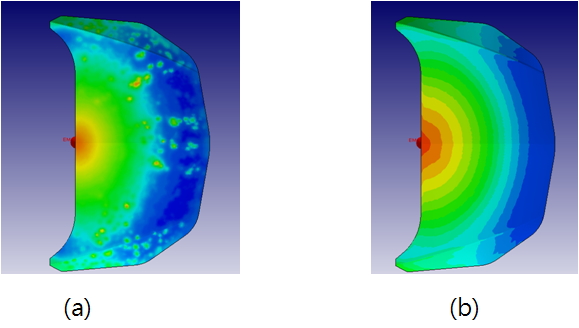
Fig. 6 (a) The simulation results before computing core enhancement, (b) The simulation results after computing core enhancement

In the RTM process, the vacuum is often used to create internal and external pressure difference and suck resin into the cavity, and at this time, the pressure at the inlet is 0.1 MPa. If a complex ply stack is used, previously, miscalculation could occur and cause the internal pressure to be higher than the maximum inlet pressure. The solver of the Moldex3D 2021 RTM module also optimizes the pressure calculation to solve this problem and obtain a reasonable pressure distribution. From the case in Fig. 7, we can see the difference before and after the enhancement of the pressure calculation for a proper maximum pressure prediction compared to inlet pressure.

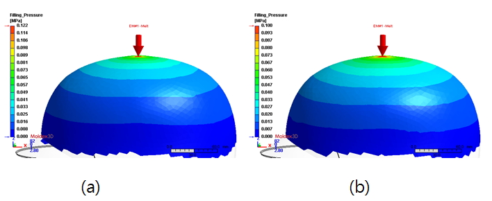
Fig. 7 (a) The maximum pressure before solver enhancement is 0.122 MPa, (b) The result after calculation solver enhancement is 0.1 MPa

Moldex3D solver supports the non-matching mesh calculation, which can reduce much of the pre-processing mesh repairing time and difficulty, helping users to quickly understand the influence of process parameters on results, and solve potential manufacturing problems earlier. In addition, the solver enhancement can provide more accurate simulation results, and improve the simulation efficiency.